Implement a Variational Autoencoder in Tensorflow

Variational autoencoders consists of an encoder and a decoder:

The encoder encodes the inputs into a posterior probability distribution over the latent variables $\mathbf{z}$, $q(\mathbf{z}|\mathbf{x})$. $q(\mathbf{z}|\mathbf{x})$ can be chosen to be a Gaussian, as such the outputs of the encoder are mean, $\boldsymbol{\mu}$, and variance, $\boldsymbol{\sigma}^2$.
A sampling step is required to sample the variables $\mathbf{z}$ from the estimated posterior density.
The decoder decodes the latent variables $\mathbf{z}$ into a representation of the input data. In case of classification, for instance, the outputs are the class labels.

It should be noted that the gradients cannot backpropagate through the model as presented above, and more specifically through the random variables $\mathbf{z}$. As a remedy, $\mathbf{z}$ is expressed as function of an additional random variable $\boldsymbol{\epsilon}$. For the sake of simplicity, $\mathbf{z}$ can be written as: $$\mathbf{z} = \boldsymbol{\mu} + \boldsymbol{\sigma}\odot\boldsymbol{\epsilon}$$.

where $\odot$ denotes a pointwise product.

The dataset

We consider the MNIST dataset that consists of 28×28 grey level images of handwritten digits. The dataset has 60000 images for training and 10000 images for testing.

Code :

from keras.datasets import mnist
# Load the MNIST data
(x_train, y_train), (x_test, y_test) = mnist.load_data()
# Scale the data
x_train = x_train.astype(“float32”) / 255
x_test = x_test.astype(“float32”) / 255

The encoder

We will code an encoder with convolutional layers. The outputs of the encoder will be fed to two fully connected layers to estimate the mean, $\boldsymbol{\mu}$, and variance, $\boldsymbol{\sigma}^2$, or more specifically $\log(\boldsymbol{\sigma}^2)$ to ensure the positivity of variance. The encoder requires setting the dimension of the latent variables $K$.

Code :

# Importing the necessary packages
from tensorflow.keras import layers, metrics, Model, backend, Sequential, callbacks, Input, losses, utils
import numpy as np
import tensorflow as tf
import matplotlib.pyplot as plt
from keras.datasets import mnist
 
class Encoder_CNN(layers.Layer):
”’
 Estimates q(z|x) using a neural net of convolutional layers
 @inputs: 
 – latent_dim: the dimension of the latent variables z
”’
def __init__(self, latent_dim=32, name=“encoder_cnn”, **kwargs):
super(Encoder_CNN, self).__init__(name=name, **kwargs)
self.encoder = Sequential(
[layers.Conv2D(32, kernel_size=(3, 3), activation=“relu”),
layers.MaxPooling2D(pool_size=(2, 2)),
layers.Conv2D(64, kernel_size=(3, 3), activation=“relu”),
layers.MaxPooling2D(pool_size=(2, 2)),
layers.Flatten(),
layers.Dropout(0.5)])
self.dense_mean = layers.Dense(latent_dim)
self.dense_log_var = layers.Dense(latent_dim)
self.sampling = Sampling()
def call(self, inputs):
”’
 @inputs: the dataset
 @Outputs: z_mean, z_log_var, and samples z
”’
x = self.encoder(inputs)
z_mean = self.dense_mean(x)
z_log_var = self.dense_log_var(x)
z = self.sampling((z_mean, z_log_var))
return z_mean, z_log_var, z

Sampling

In the code above there is a sampling step that consists of sampling the latent variables from the estimated distribution $q(\mathbf{z}|\mathbf{x})$. This step uses the reparametrization trick that ensures the backpropagation of the gradients. This step involves the formulation of $\mathbf{z}$ as function of $\boldsymbol{\epsilon}$.

Code :

class Sampling(layers.Layer):
”’
 Samples the latent variables z given the z_mu and z_log_var outputs of 
 the encoder and using the reparameterization trick
”’
def __init__(self):
super().__init__()
def call(self, inputs):
# Extract the inputs
z_mu, z_log_var= inputs
# Get the noise epsilon
eps = backend.random_normal(shape = tf.shape(z_mu), stddev=1e-4)
return z_mu + backend.exp(0.5*z_log_var)*eps

The decoder

The decoder does not have to mirror the encoder, but I made it that way.

Code :

class Decoder_CNN(layers.Layer):
”’
 Estimates p(x|z)
”’
def __init__(self, name=“decoder_cnn”, **kwargs):
super(Decoder_CNN, self).__init__(name=name, **kwargs)
self.decoder = Sequential([layers.Dense(1600),
layers.Reshape((5, 5, 64)),
layers.UpSampling2D(2),
layers.Conv2DTranspose(64, 3, activation=“relu”),
layers.UpSampling2D(2),
layers.Conv2DTranspose(32, 3, activation=“relu”),
layers.Conv2DTranspose(1, 3, activation=“sigmoid”)])
def call(self, inputs):
”’
 @inputs: the latent variables z
 @outputs: the reconstructed data
”’
return self.decoder(inputs)

The loss function

The loss function writes, (for more details check here)

$$\mathcal{L}(\mathbf{x}) = \mathbb{E}_q\Big[\log\big(p(\mathbf{x}, \mathbf{z}) \big) – \log\big(q(\mathbf{z}| \mathbf{x})\big)\Big] = \mathbb{E}_q\Big[\log\big(p(\mathbf{x}|\mathbf{z}) \big)\Big] – D_{KL}\big(q(\mathbf{z}|\mathbf{x})||p(\mathbf{z})\big)$$

It consists of two terms.

The first term depends on the data’s distribution. The MNIST dataset is binary (background in black and digits in white), accordingly it can be modeled by a Bernoulli distribution. In this case, $\mathbb{E}_q\Big[\log\big(p(\mathbf{x}|\mathbf{z}) \big)\Big]$ is given by the binary cross entropy available in Keras.
The second term is the Kullback Leibler divergence between $q(\mathbf{z}|\mathbf{x})$ and $p(\mathbf{z})$, which are both Gaussians. We assume that $p(\mathbf{z}) = \mathcal{N}\left(\mathbf{0}, \mathbf{I}\right)$, accordingly,

$$D_{KL}\big(q(\mathbf{z}|\mathbf{x})||p(\mathbf{z})\big) = \frac{1}{2} \sum_{k=1}^K \Big( -1 + \boldsymbol{\mu}^2_k + \boldsymbol{\sigma}^2_k – \log\big(\boldsymbol{\sigma}^2_k\big)\Big)$$

Putting everything together!

We combine the encoder and decoder together.

Code :

class VariationalAutoEncoder(Model):
”’
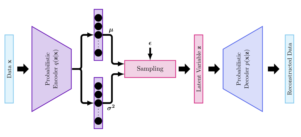
 Combines the encoder and decoder into an one model for training and adds the KL regularization term to the loss.
”’
def __init__(
self,
original_dim,
intermediate_dim=64,
latent_dim=32,
name=“vae_autoencoder”,
**kwargs
):
super(VariationalAutoEncoder, self).__init__(name=name, **kwargs)
self.loss_tracker = tf.keras.metrics.Mean(name=‘loss’)
self.original_dim = original_dim
self.encoder = Encoder_CNN(latent_dim=latent_dim)
self.decoder = Decoder_CNN()
self.shape = (28, 28, 1)
def call(self, inputs):
# Encoder
z_mean, z_log_var, z = self.encoder(inputs)
# Adding the KL term to the loss
kl_loss = – .5 * backend.sum(1 + z_log_var –
backend.square(z_mean) –
backend.exp(z_log_var), axis=-1)
self.add_loss(backend.mean(kl_loss))
# Decoder
reconstructed = self.decoder(z)
return reconstructed
def train_step(self, data):
x, y , _ = utils.unpack_x_y_sample_weight(data)
with tf.GradientTape() as tape:
x_decoded = self(x)
loss = self.compute_loss(y = y, y_pred = x_decoded)
self.optimizer.minimize(loss, self.trainable_variables, tape=tape)
return self.compute_metrics(x, y, x_decoded, None)
def compute_loss(self, x=None, y=None, y_pred=None, sample_weight=None):
loss = backend.sum(backend.mean(losses.binary_crossentropy(y, y_pred), axis = 0))
loss += tf.add_n(self.losses)
self.loss_tracker.update_state(loss)
return loss

Let's run the code!

# Make sure images have shape (28, 28, 1)
x_train = np.expand_dims(x_train, -1)
x_test = np.expand_dims(x_test, -1)

# VAE
latent_dim = 10
batch_size = 128
epochs = 200
data_dim = (28,28,1)

stop_early = callbacks.EarlyStopping(monitor=‘val_loss’, patience=5)
vae = VariationalAutoEncoder(data_dim, latent_dim = latent_dim)
x = Input(data_dim)
z_mean, _, z = vae.encoder(x)
x_decoded = vae.decoder(z)
vae.compile(optimizer=‘adam’)
vae.fit(x_train,
x_train,
shuffle=True,
epochs=epochs,
batch_size=batch_size,
validation_data=(x_test, x_test),
callbacks = stop_early)

Below we show the t-SNE (t-distributed Stochastic Neighbor Embedding) of the original dataset MNIST and the corresponding embeddings $\mathbf{z}$. Note how the embeddings improve the classes’ separation.

Original digits and reconstructed digits by the implemented VAE

Was this post useful? Let me know what do you think about it below…

The dataset

Code :

The encoder

Code :

Sampling

Code :

The decoder

Code :

The loss function

Putting everything together!

Code :

Let's run the code!

Related posts:

Leave a Comment Cancel Reply